

What is the population of that region?
I have been working on a game that simulates high-speed train networks. For realistic ridership estimates, I need to compute how many people live near a station.
City or metro populations would work, but allowing user-defined definitions based on populations within some radius allows for more consistency and flexibility. After downloading gridded population of the world data from the ESDS program at NASA, I ended up having a lot of fun exploring some questions about population distributions.
- How many people live within a circle of a given radius?
- How large of a circle is needed to reach a given population?
- What direction leads to the center of population?
- Where is the enclosing contour of a given density?
- How many people live close to each ocean?
- How many people live in particular climates?
The population data are estimates of 2020 populations and I've tried to be as accurate as the underlying data allows. I wasn't looking for a definitive answer to any particular question so I mostly made lots of pretty pictures and charts without regard for things like error bars.
Computation Considerations
Most of the hard work has been done as it is possible to download one file to get detailed data for every region of Earth. Using cells with a height and width of 1/24th of a degree (roughly 5 km x 5 km near the equator) is accurate enough for my purposes, but they also offer a dataset down to 1/120th of a degree.
Haversine formula for distance
The Earth is neither flat nor a perfect sphere, so depending on the accuracy required there are several possible formulas to compute the distance between two points.
The haversine formula is fast, simple, and accurate within 1% for any pair of endpoints. For any sphere, the distance between two points can be computed as
where r is the radius, are the latitudes, and are the longitudes. A perfect sphere with the same volume as the Earth would have a radius of around 6371 km (3959 miles), and using this value for the radius produces good estimates anywhere.
function haversine(lat1,lon1,lat2,lon2) {
       //convert to radians (*Math.PI/180) if in degrees
       var R = 6371; // avg radius of the Earth in km
       var dLat = lat2 - lat1; var dLon = lon2 - lon1;
       var a = Math.sin(dLon / 2) * Math.sin(dLon /2);
       a *= Math.cos(lat1) * Math.cos(lat2);
       a += Math.sin(dLat / 2) * Math.sin(dLat /2);
       return 2 * Math.asin(Math.sqrt(a)) * R;
}
Area
This answer walks through the computation of the area of a gridded rectangle on the surface of a sphere. The area is
where r is again 6371 km and the longitudes ( ) are in degrees.
Since I am working with squares of the same size in terms of latitude/longitude, I can make some simplifying assumptions for the area so the function requires just one input: the average latitude.
function area(lat){
  let c = 1/24;//each square is 1/24 of a degree
  let R = 6371;
  let lat1 = (lat-c/2)*Math.PI/180;//radians for bottom
  let lat2 = (lat+c/2)*Math.PI/180;//radians for top
  let x = Math.sin(lat2)-Math.sin(lat1);//lat2>lat1
  return 2*Math.PI*R*R*x*(c/360);
}
Population within a given radius
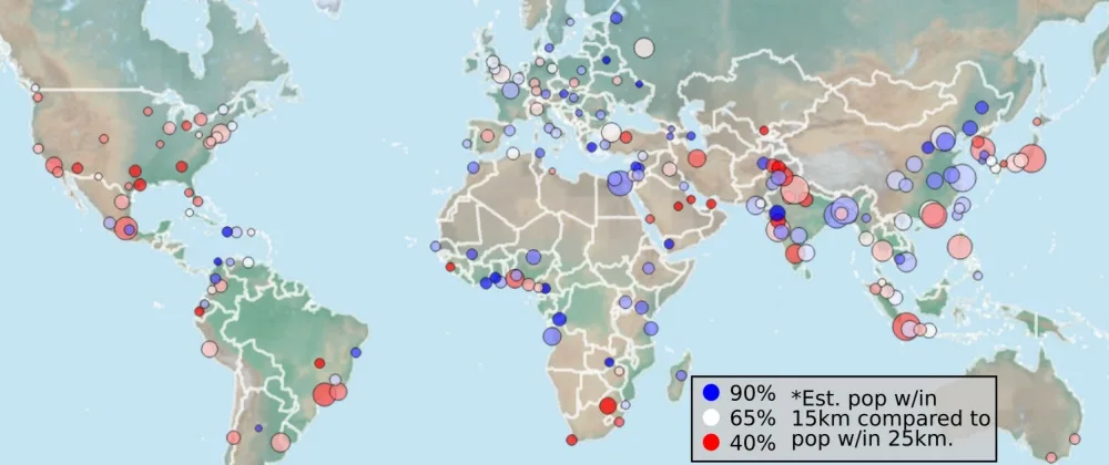
To compute the population within a particular circle, I determine which squares are completely inside the circle, partially contained, and completely outside. I then compute the total population and total area of this circle-like region and multiply that population density by the area of the circle.
This computation is relatively quick for one circle, but to create a map we need to perform this calculation tens of thousands of times. The simplest optimization is to reuse as much of each circle as possible.
Working row-by-row, the circles move one unit for each pixel. After computing the first circle in a row we save lots of calculations and look-ups by just computing the differences for subsequent columns. Don't forget the wrap-around at the International Date Line, though.
You can create a map like the one below with a custom radius by forking this repository on Replit.
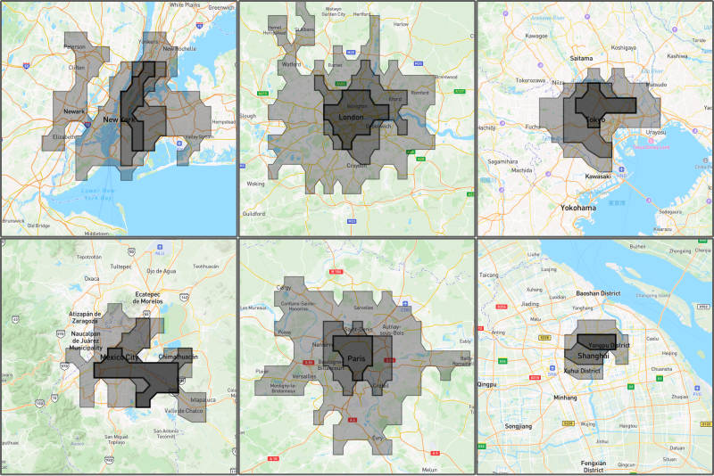
Selected Cities
My original intent was about populations close to cities, and I ran some calculations for 200 geographically diverse large cities. Using a simple radius-based computation allows for some consistent comparisons, but people who live the same distance from a city center can still have very different connections to that city depending on the locations of surrounding cities and transit connectivity.
Although Tokyo is generally considered to have the largest population of any metropolitan area, Shanghai has a very dense core and Delhi seems to have a larger population within 50km.
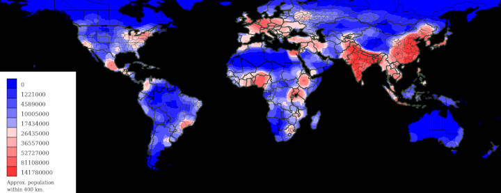
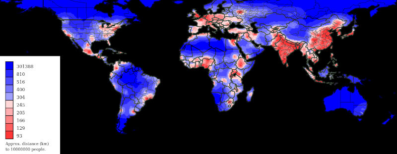
Distance to a given population
An interesting related question is to determine how large of a circle is required to enclose a certain population. The fastest way to get this answer for one population would be some sort of binary search.
Reusing circles when computing the radius for every pixel saves a lot of time, but there is less flexibility to use custom radii. I ended up using a fixed array of possible circles and then interpolated in between to arrive at the answers.
If the population within 50 km is 7 million and the population within 100 km is 13 million, at what radius is the population likely to be 10 million? One guess is to take a linear average and guess 75 km. This guess is more than good enough to make the algorithm converge quickly, but we should probably account for the fact that area increases with the square of the radius.
Another approach is to assume the band between 50 km and 100 km has uniform density and then compute the radius as . For a circle around a major city, this band might have decreasing population density making this guess worse than the linear average.
A Calculus-based approach might be even better, but that would involve solving a cubic equation. If you are looking for a fun volume of revolutions integration question (and who isn't?), then try to solve the above based on various assumptions about how the population density declines from the center to the edge.
The map we produce is quite similar to the one above, but more large cities become visible. The main advantage of this calculation would be dealing with multiple data points. Per capita computations can be wonky when the denominator varies wildly, so uniform populations should remove a lot of outliers (which may or may not be good).
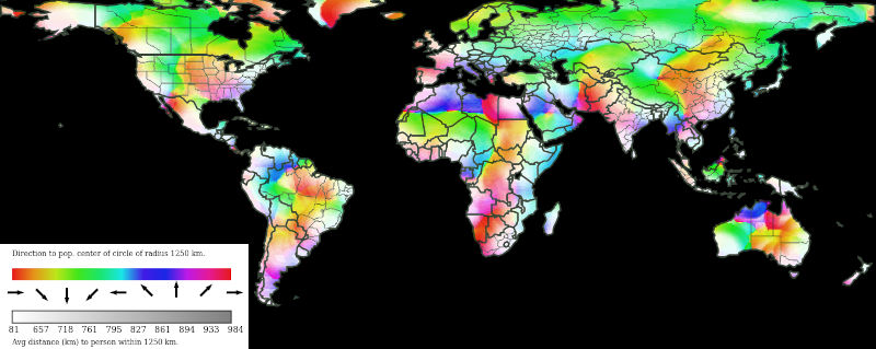
Direction to population center
While computing the total population within a circle, we can also compute the center of mass. For each grid cell, we determine the population-weighted x and y distances to the center of the circle. Then we can compute averages and find the angle with the arctangent function.
let pop = 0, x = 0, y = 0;
let center = {x:0,y:0};//the center of the circle
let circle = {...};//points in the circle around center
for (var cell in circle){
  pop += cell.pop;
  let xdiff = cell.x-center.x;
  let ydiff = cell.y-center.y;
  x += cell.pop*xdiff;
  y += cell.pop*ydiff;
}
let angle = Math.atan2(y/pop,x/pop)*180/Math.PI;
if (angle < 0){angle += 360}
let distance = Math.sqrt(Math.pow(y/pop,2)+Math.pow(x/pop,2));
When mapping angles, we do need a method that wraps around to make 0° equal 360°. I use the HSL color space because the hue attribute does exactly this with red occupying both ends. I can then use lightness to show the distance to the center of mass. I'm not sure what it all means, but I thought the maps looked cool.
Contours of population density
Different cities and regions can have very different population distributions based on the locations of water, mountains, and many other natural or human influences. By setting the correct minimum population density, we can find small regions with a given total population using contours.
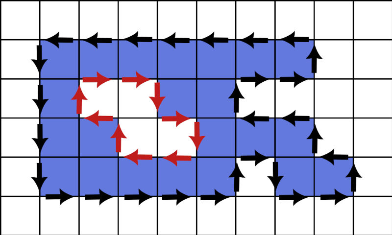
The first step is to generate a binary mask with cells either being 1 or 0 depending on whether their population density is higher than some cutoff value. Then we can use a contour-finding algorithm to separate regions of 1s versus 0s. The algorithm has three parts:
- Find an outside wall dividing a 1 and a 0.
- Walk along the wall, keeping it on your left.
- Stop when you repeat a previous state.
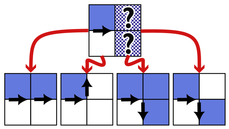
This algorithm of always keeping the wall on your left (or right, but choose one direction) also solves many mazes. It is very simple as long as you keep track of the direction you are traveling.
To find our starting points we just look for a 0 on top of a 1. Since a map may have many contours, we will keep track of which cells we visit and skip over any potential starting points that have already been visited in the same direction. I haven't proven anything, but I believe all contours and any holes within will eventually be found.
To walk along the wall we need to know our location and the direction we came from. Then we check whether two neighboring cells are 1s or 0s to determine our next move. I choose to include diagonally adjacent squares in the same region, but you could modify the last option below to do the opposite.
I terminate when I reach a square that I have visited before in the same direction. After this point, the algorithm would just repeat forever. Then I check if there is another starting point and repeat until there are no more contours or holes.
Identifying holes doesn't require doing anything special, but we end up going clockwise. If creating an SVG path, then the renderer can automatically leave these holes unfilled. I also took the easy route of using the isPointInFill() function to determine which cells are within a contour to compute total populations.
If you wish to watch the algorithm find custom contours for North America or the world, enter a minimum population density in the Codepen below.
Coastal Populations
I thought it would be easy to download shapefiles for the oceans of the world, but I could not find anything that worked right. I ended up downloading a set from Natural Earth with more than 100 seas/oceans and then merged many of them into a collection of twelve that seemed reasonable.
The values for the global coastline are relatively straightforward, but I have left it up to you to pick which seas among this list should be counted as part of which oceans. In the future, I hope to make it possible to pick the coastlines with much more granularity to look at something like the Atlantic coast of the United States.
I do want to extend the idea to calculate populations within some distance of a variety of natural regions. Along with getting the right datasets for rivers, lakes, mountain ranges, and more, I need faster and more accurate methods of computing populations within arbitrary polygons.
Weather and Population
I downloaded weather data from 2011-2020 for each 0.5°x0.5° block from the Climate Research Unit at the University of East Anglia. Their monthly data includes average temperatures, low and high temps, diurnal ranges, vapor pressure, wet days, precipitation, and frost days.
I wanted to create some sort of neural net to predict population density based on weather, but the results were subpar. Nearby cells have very similar populations and weather, so you need to do something like using Eastern Hemisphere data to predict the Western Hemisphere. When I used my basic machine learning skills I could not do better than a simple temperature-based prediction. If you wish to try, you can download this csv (6 MB) that includes population and weather data.
Click any populated area in the map below and see how similar the weather is everywhere else. For similarity, I am using Euclidean distance with equal weights to each of eight normalized characteristics (six are temp-based and two are precipitation).
You can also enter your latitude and longitude to generate a radar chart to visualize where your location ranks across the eight statistics. I have computed population-weighted mean, standard deviation, and decile cutoffs for each statistic to allow for decent comparisons in most situations.
Analyzing weather is a scenario where a simple population density ( ) actually might be superior to a population-weighted density ( ). However, without data for unpopulated areas, I decided to use the population-weighted density anyway because those cells do not factor into the calculation.
Make Your Own Maps
If you want to download the raw population data, it comes as a geoTIFF and I found Python's libraries easiest for reading and analyzing geometric data. In particular, here is the code I used to produce a data frame from the tiff.
import rioxarray
import pandas

rds = rioxarray.open_rasterio(filename,)
rds = rds.squeeze().drop("spatial_ref").drop("band")
rds.name = "data"
df = rds.to_dataframe().reset_index()
For simpler questions, fork this repository on Replit to generate maps of population within a radius, radius to a given population, and the center of population for custom values. Or view the other related repositories in my portfolio.